Method of Characteristics
The method of characteristics is a technique wherein a partial differential equation is reduced to a family of ordinary differential equations along which the solution can be integrated from some initial data. Typically, it applies to first-order equations although more generally the method of characteristics is valid for any hyperbolic partial differential equation.
In classifying the difference in behaviour between elliptic, parabolic and hyperbolic PDEs the existing of characteristic curves is a key feature in this classification. Namely parabolic and hyperbolic PDEs, that describe a system that evolves in time, have characteristic curves along which the solution evolves with the information propagating along them travelling away from the given initial conditions. This is in contrast to elliptic PDEs that do not have characteristic curves and thus no real sense of information propagation.
In order to talk properly about characteristics we look at linear homogenous hyperbolic wave equation as an example.
$$\frac{\partial^2u}{\partial t^2} - c^2 \frac{\partial^2u}{\partial x^2} = 0 \phantom{xxxxxxxxx}(1)$$
The wave equation (1) can be refactored in the following two ways:
$$\Big(\frac{\partial}{\partial t} + c\frac{\partial}{\partial x}\Big)\Big( \frac{\partial u}{\partial t} - c\frac{\partial u}{\partial x}\Big) = 0$$
$$\Big(\frac{\partial}{\partial t} - c\frac{\partial}{\partial x}\Big) \Big(\frac{\partial u}{\partial t} +c\frac{\partial u}{\partial x}\Big) = 0$$
since the mixed second derivative terms vanish in both. If we let
$$w = \frac{\partial u}{\partial t} - c\frac{\partial u}{\partial x}\phantom{xxxxxxxxx}(2)$$
$$v = \frac{\partial u}{\partial t} + c\frac{\partial u}{\partial x}\phantom{xxxxxxxxx}(3)$$
we see that the one-dimensional wave equation (1), involving second derivatives, yields two first-order wave equations:
$$\frac{\partial w}{\partial t} + c\frac{\partial w}{\partial x} = 0 \phantom{xxxxxxxxx}(4)$$
$$\frac{\partial v}{\partial t} - c\frac{\partial v}{\partial x} = 0 \phantom{xxxxxxxxx}(5)$$
Taking (4) we look to apply the method of characteristics such that the first-order PDE reduces to a family of ordinary differential equations. The method is applied by considering the rate of change of \(w(x(t),t)\) as measured by a moving observer, \(x=x(t)\). Applying the chain rule we find
$$\frac{d}{dt}w(x(t),t) = \frac{\partial w}{\partial t} + \frac{dx}{dt} \frac{\partial w}{\partial x} \phantom{xxxxxxxxx}(6)$$
The first term \(\frac{\partial w}{\partial t}\) represents the change in \(w\) at the fixed position, while \(\frac{dx}{dt} \frac{\partial w}{\partial x}\) represents the change due to the fact that the observer moves into a region of possibly different \(w\). Compare (6) with the partial differential equation for \(w\) in (4). It is apparent that if the observer moves with velocity \(c\), that is, if:
$$\frac{dx}{dt}=c\phantom{xxxxxxxxx}(7)$$
then
$$\frac{dw}{dt}=0\phantom{xxxxxxxxx}(8)$$
Thus \(w\) is constant. Therefore an observer moving with this special speed \(c\) would measure no changes in \(w\).
In this way, the partial differential equation (4) has been replaced by two ordinary differential equations, (7) and (8). Integrating (6) yields
$$x=ct+x_0\phantom{xxxxxxxxx}(9)$$
the equation for the family of parallel characteristics of (4), sketched in Fig 1. Note that at \(t=0,x=x_0. w(x,t)\) is constant along this line. \(w\) propagates as a wave with wave speed \(c\).
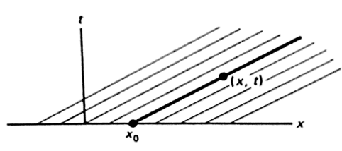
Fig 1 : Characteristics for the first order wave equation
If \(w(x,t)\) is given initially at \(t=0\),
$$w(x,0)=P(x)\phantom{xxxxxxxxx}(10)$$
then let us determine \(w\) at the point \(x,t\). Since \(w\) is constant along the characteristic,
$$w(x,t)=w(x_0,0)=P(x_0)\phantom{xxxxxxxxx}(11)$$
Given \(x\) and \(t\), the parameter is known from the characteristic, \(x_0=x-ct\) and thus
$$w(x,t)=P(x-ct)\phantom{xxxxxxxxx}(12)$$
which we call the general solution of (4).
We can think of \(P(x)\) as being an arbitrary function. To verify this, we substitute (12) back into the partial differential equation (4). Using the chain rule
$$\frac{\partial w}{\partial x} =\frac{dP}{d(x-ct)}\frac{\partial (x-ct)}{\partial x}=\frac{dP}{d(x-ct)}\phantom{xxxxxxxxx}(13)$$
and
$$\frac{\partial w}{\partial t} = \frac{dP}{d(x-ct)}\frac{\partial (x-ct)}{\partial t}=-c\frac{dP}{d(x-ct)}\phantom{xxxxxxxxx}(14)$$
Thus, it is verified that (4) is satisfied by (12). The general solution of a first-order partial differential equation contains an arbitrary function, while the general solution to the ordinary differential equations contains arbitrary constants.